Projects Executed
Choosing Mechanical Engineering for graduation was almost like a reflex and it proved to be one of my greatest technical learning experiences. My major work was my final semester bachelor’s dissertation. As a part of my final semester project at NIT Silchar, I worked on two problems based on computational fluid dynamics which were:
Choosing Mechanical Engineering for graduation was almost like a reflex and it proved to be one of my greatest technical learning experiences. My major work was my final semester bachelor’s dissertation. As a part of my final semester project at NIT Silchar, I worked on two problems based on computational fluid dynamics which were:
- Obtaining an optimum hovering condition in terms of blade rotational speed and the angle of attack of the rotor’s aerofoil
- Analyzing flow around isolated wings of the Airbus A380 during flight modes and comparing with the high lift S1223 aerofoil.
CFD analysis of an isolated main helicopter rotor for a hovering flight at varying RPM
Abstract:
The main objective of the simulation was to analyze the flow around an isolated main helicopter rotor at various main rotor speed of 800, 600 and 400 RPM at an angle of attack of 8 degrees using the blade profile of Eurocopter AS350B3. The Eurocopter AS350B3 uses the blade profile of standard ONERA OA209 airfoil. Analysis was done for the hovering flight condition and comparison of stability in terms of wake formations and vorticity was performed. The parameters helped in obtaining an optimum RPM at an angle of attack of 8 degrees during hovering. For the analysis, the moving reference frame (MRF) method with the standard viscous K-Î turbulent flow model was used. The model is quite popular for such problems on the account of its accuracy.
Modelling:
GAMBIT was used for the 3D design of the computational domain according to the following steps:
The appropriate computational domain was made and selection of boundary conditions was fixed based on a simulation performed at Georgia Institute of Technology (GIT) on simulating rotor wake and body interaction. The larger ratio between computational domain and rotor size was used to minimize the blockage effect or wall boundary effect particularly below the rotating rotor where the airflow is induced downstream by the rotor. The appropriate height between the rotor and the bottom wall boundary is important because it may increase the ground effect on the rotor performance.
In pre-processing stage, the blade was meshed using edge and face meshing in order to take care of the skewness. T-Grid type of mesh and Tet/Hex elements made 1222765 cells (2467458 faces) and 214798 nodes for the domain. It was used in order to have better accuracy. But using the finer mesh requires smaller time steps, more number of iterations per time step and 4 times more calculation per iteration for the solution to converge.
The GAMBIT software comes with different boundary types which synchronize with the physical conditions. The FLUENT 5/6 boundary model was incorporated which uses the ‘VELOCITY INLET’ boundary types for air inlet. For the outlet condition, ‘PRESSURE OUTLET’ boundary condition was used. Pressure and velocity conditions were as in the normal atmospheric conditions. The rest of the regions were defined as ‘WALL’ boundary type, for e.g., the blade and the domain walls.
Simulation:
After the meshing was completed and the suitable boundary types were defined in GAMBIT, the model was then imported into FLUENT 6.3 using 3-D SOLVER. The finite volume approach was used in CFD, which is used to create the solver. The governing equations are then integrated over the whole control volume (the computational domain is divided into a finite quantity of small cells, each of which acts as an individual control volume). The turbulent model used was the k-ε turbulence model suggested by Launder and Spalding. The Moving Reference Frame (MRF) method was used for the simulation of fluid flow over the rotor blades during hovering flight condition. A pressure based implicitly steady solver was selected and the velocity formulation was set to absolute. The discretization scheme for momentum, turbulence kinetic energy and turbulence dissipation rate were all second order upwind and the pressure-velocity coupling scheme was set to SIMPLE. The solution was initialized from velocity inlet. For accurate prediction of the effects of turbulence in the boundary layer on the blades, boundary layers were formed. Boundary layers are the layers of elements growing out from a boundary into the domain. They are used to locally refine the mesh in the direction normal to a face or an edge. The height of the first cell adjacent to a solid boundary must satisfy eqn. shown below for accurate prediction of the skin friction in a boundary layer,
(Δn)u*/νω≤1 (1)
Where, Δn is the height of the first cell adjacent to the solid boundary, u* is the friction velocity and νω is the kinematic viscosity. 8 numbers of rows were selected with 0.001 as the magnitude of the first row (i.e. the height of the first row of elements normal to the edge) and the growth factor was set to 1.05 (This sets the ratio of distances between consecutive rows of elements.). From the above two parameters the depth found was 0.00954911 in magnitude (The depth is the total height of the boundary layer).
Convergence of the solution:
Convergence and accuracy is important during solution. If not then we have to change the solution parameters and sometimes solution method also. The residuals were calculated for a number of mesh cells and after calculating the residuals for each amount of mesh cells (say 1e6, 2e6, 6e6, 12e6 etc., where the magnitudes represent the amount of mesh cells, i.e. the number of cells generated) it was found that the residuals limit to a particular value even when the mesh cells are increased further, therefore in order to optimize the memory requirement and the computational time, the mesh elements were decided accordingly. The residual for various parameters were found to be in a range which was good enough to place our confidence on the converged solution.
Conclusion:
From the analysis it was obtained that at a speed of 400 RPM wake formation and tip vorticity is low thus affecting the lift of the helicopter resulting in a steady hovering. Also due to this lower tip vorticity, noise of the blades is reduced (refer fig. below).
Abstract:
The main objective of the simulation was to analyze the flow around an isolated main helicopter rotor at various main rotor speed of 800, 600 and 400 RPM at an angle of attack of 8 degrees using the blade profile of Eurocopter AS350B3. The Eurocopter AS350B3 uses the blade profile of standard ONERA OA209 airfoil. Analysis was done for the hovering flight condition and comparison of stability in terms of wake formations and vorticity was performed. The parameters helped in obtaining an optimum RPM at an angle of attack of 8 degrees during hovering. For the analysis, the moving reference frame (MRF) method with the standard viscous K-Î turbulent flow model was used. The model is quite popular for such problems on the account of its accuracy.
Modelling:
GAMBIT was used for the 3D design of the computational domain according to the following steps:
- The ONERA standard airfoil OA209 was selected for the rotor blades.
- The angle of attack was fixed at 8 degrees based on a moderate normal collective pitch for a hovering flight for initial simulation.
The appropriate computational domain was made and selection of boundary conditions was fixed based on a simulation performed at Georgia Institute of Technology (GIT) on simulating rotor wake and body interaction. The larger ratio between computational domain and rotor size was used to minimize the blockage effect or wall boundary effect particularly below the rotating rotor where the airflow is induced downstream by the rotor. The appropriate height between the rotor and the bottom wall boundary is important because it may increase the ground effect on the rotor performance.
In pre-processing stage, the blade was meshed using edge and face meshing in order to take care of the skewness. T-Grid type of mesh and Tet/Hex elements made 1222765 cells (2467458 faces) and 214798 nodes for the domain. It was used in order to have better accuracy. But using the finer mesh requires smaller time steps, more number of iterations per time step and 4 times more calculation per iteration for the solution to converge.
The GAMBIT software comes with different boundary types which synchronize with the physical conditions. The FLUENT 5/6 boundary model was incorporated which uses the ‘VELOCITY INLET’ boundary types for air inlet. For the outlet condition, ‘PRESSURE OUTLET’ boundary condition was used. Pressure and velocity conditions were as in the normal atmospheric conditions. The rest of the regions were defined as ‘WALL’ boundary type, for e.g., the blade and the domain walls.
Simulation:
After the meshing was completed and the suitable boundary types were defined in GAMBIT, the model was then imported into FLUENT 6.3 using 3-D SOLVER. The finite volume approach was used in CFD, which is used to create the solver. The governing equations are then integrated over the whole control volume (the computational domain is divided into a finite quantity of small cells, each of which acts as an individual control volume). The turbulent model used was the k-ε turbulence model suggested by Launder and Spalding. The Moving Reference Frame (MRF) method was used for the simulation of fluid flow over the rotor blades during hovering flight condition. A pressure based implicitly steady solver was selected and the velocity formulation was set to absolute. The discretization scheme for momentum, turbulence kinetic energy and turbulence dissipation rate were all second order upwind and the pressure-velocity coupling scheme was set to SIMPLE. The solution was initialized from velocity inlet. For accurate prediction of the effects of turbulence in the boundary layer on the blades, boundary layers were formed. Boundary layers are the layers of elements growing out from a boundary into the domain. They are used to locally refine the mesh in the direction normal to a face or an edge. The height of the first cell adjacent to a solid boundary must satisfy eqn. shown below for accurate prediction of the skin friction in a boundary layer,
(Δn)u*/νω≤1 (1)
Where, Δn is the height of the first cell adjacent to the solid boundary, u* is the friction velocity and νω is the kinematic viscosity. 8 numbers of rows were selected with 0.001 as the magnitude of the first row (i.e. the height of the first row of elements normal to the edge) and the growth factor was set to 1.05 (This sets the ratio of distances between consecutive rows of elements.). From the above two parameters the depth found was 0.00954911 in magnitude (The depth is the total height of the boundary layer).
Convergence of the solution:
Convergence and accuracy is important during solution. If not then we have to change the solution parameters and sometimes solution method also. The residuals were calculated for a number of mesh cells and after calculating the residuals for each amount of mesh cells (say 1e6, 2e6, 6e6, 12e6 etc., where the magnitudes represent the amount of mesh cells, i.e. the number of cells generated) it was found that the residuals limit to a particular value even when the mesh cells are increased further, therefore in order to optimize the memory requirement and the computational time, the mesh elements were decided accordingly. The residual for various parameters were found to be in a range which was good enough to place our confidence on the converged solution.
Conclusion:
From the analysis it was obtained that at a speed of 400 RPM wake formation and tip vorticity is low thus affecting the lift of the helicopter resulting in a steady hovering. Also due to this lower tip vorticity, noise of the blades is reduced (refer fig. below).
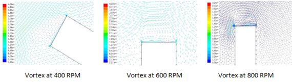
However, it was observed that the magnitude of the vortex formation and the resulting wake starts increasing with the increase in RPM (refer fig. above). It reaches its maximum at 800 RPM in our analysis, as a result of which maximum energy loss is predicted on the account of the wake formation and loading on the engine would increase significantly. Thus from the analysis a main rotor speed of 400 RPM may provide the desirable conditions for a steady hovering operation of a helicopter. It was found from the study that the simulation method used was capable of providing good simulation results within the error limits that may be utilized in understanding the wake formation and its effect on the lift produced by the blades, the dynamic motion would be included in the future study on simulating a complete helicopter aerodynamics performance.
To see the publication details click here
To see the publication details click here
CFD analysis of Airbus A380 isolated wings during take-off, cruising and landing and comparison with low Reynold’s number, high lift S1223 airfoil
Abstract:
This project presents a numerical analysis of the Airbus A380 passenger aircraft using the computational model of the isolated wings of Airbus A380 during take-off, cruising and landing conditions which were developed using GAMBIT and simulated using FLUENT. The present aircraft wing section which is made up of a blend of NASA SC(2)_0610 and NASA SC(2)_0606 airfoils have been compared with a low Reynold’s number, high lift S1223 airfoil, 3D analysis of the proposed model was performed. It was found that the selected S1223 airfoil gives comparatively better results under simple configurations i.e. without effects of slats and flaps. Lift and drag coefficients were calculated for different conditions.
Modelling:
In the design environment of GAMBIT 2.3.16, the 3D design of computational domain was developed following the steps below:
For the CFD analysis, the computational domain used was a simple rectangular control volume. Here wall effects are not a part of the study and also it does not affect the study reasonably. A simple control volume configuration was selected so as to simplify the calculation efforts and make it more efficient and economic in terms of computational time. In pre-processing stage, the wings were designed and meshed using edge and face meshing in order to take care of the skewness. The domain was meshed using tetrahedral meshing technique.
The GAMBIT 2.3.16 software comes with different boundary types which synchronize with the physical conditions. The FLUENT 6.3.26 boundary model was incorporated which uses the ‘VELOCITY INLET’ boundary types for air inlet. For the outlet conditions ‘OUTFLOW’ boundary condition was used. Pressure and velocity conditions were as in the normal atmospheric conditions. The wings surface was defined as ‘WALL’ boundary type and that of the wind tunnel as ‘SYMMETRY’ boundary type.
Simulation:
After the meshing was completed and suitable boundary types were defined in GAMBIT 2.3.16, the model was then exported to FLUENT 6.3.26 using 3DDP SOLVER. The finite volume approach was used to create the solver. The governing equations were then integrated over the whole control volume (the computational domain being divided into finite quantity of small cells, each of which acts as an individual control volume). The k-ε turbulence model was used. Criteria used for boundary layer were same as explained for the project on CFD analysis for a rotorcraft above.
Conclusion:
The CFD analysis of Airbus A380 isolated wings presented satisfactory results which were in agreement with the expected conditions for the same. The flying characteristics in terms of dynamic pressure and turbulent viscosity for present airfoil was analyzed and also compared with S1223 airfoil.
Abstract:
This project presents a numerical analysis of the Airbus A380 passenger aircraft using the computational model of the isolated wings of Airbus A380 during take-off, cruising and landing conditions which were developed using GAMBIT and simulated using FLUENT. The present aircraft wing section which is made up of a blend of NASA SC(2)_0610 and NASA SC(2)_0606 airfoils have been compared with a low Reynold’s number, high lift S1223 airfoil, 3D analysis of the proposed model was performed. It was found that the selected S1223 airfoil gives comparatively better results under simple configurations i.e. without effects of slats and flaps. Lift and drag coefficients were calculated for different conditions.
Modelling:
In the design environment of GAMBIT 2.3.16, the 3D design of computational domain was developed following the steps below:
- The NASA standard airfoil NASA SC(2)_0610 and NASA SC(2)_0606 was selected for the design of the isolated wings.
- The high lift S1223 aerofoil was selected for the design of isolated wings for comparison.
For the CFD analysis, the computational domain used was a simple rectangular control volume. Here wall effects are not a part of the study and also it does not affect the study reasonably. A simple control volume configuration was selected so as to simplify the calculation efforts and make it more efficient and economic in terms of computational time. In pre-processing stage, the wings were designed and meshed using edge and face meshing in order to take care of the skewness. The domain was meshed using tetrahedral meshing technique.
The GAMBIT 2.3.16 software comes with different boundary types which synchronize with the physical conditions. The FLUENT 6.3.26 boundary model was incorporated which uses the ‘VELOCITY INLET’ boundary types for air inlet. For the outlet conditions ‘OUTFLOW’ boundary condition was used. Pressure and velocity conditions were as in the normal atmospheric conditions. The wings surface was defined as ‘WALL’ boundary type and that of the wind tunnel as ‘SYMMETRY’ boundary type.
Simulation:
After the meshing was completed and suitable boundary types were defined in GAMBIT 2.3.16, the model was then exported to FLUENT 6.3.26 using 3DDP SOLVER. The finite volume approach was used to create the solver. The governing equations were then integrated over the whole control volume (the computational domain being divided into finite quantity of small cells, each of which acts as an individual control volume). The k-ε turbulence model was used. Criteria used for boundary layer were same as explained for the project on CFD analysis for a rotorcraft above.
Conclusion:
The CFD analysis of Airbus A380 isolated wings presented satisfactory results which were in agreement with the expected conditions for the same. The flying characteristics in terms of dynamic pressure and turbulent viscosity for present airfoil was analyzed and also compared with S1223 airfoil.
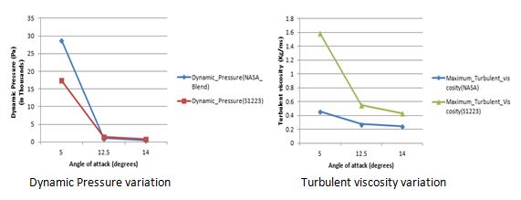
From the obtained values of dynamic pressure and turbulent viscosity it was seen that the range of dynamic pressure during cruise (angle of attack of 5 degrees) is less in case of S1223 airfoil as compared to the NASA blended airfoil (refer figure) , which is also one of the most desirable effects as during lower angle of attack, the effective number of molecular collision is lesser that can produce dynamic pressure, therefore here static pressure would be dominating factor of the two components, i.e. the dynamic and static pressure contribute to the total pressure and as the dynamic pressure is low in case of S1223; more of the components would be static which would contribute to the total pressure, this makes the performance for the S1223 airfoil better as compared to the NASA blended airfoil.
For higher angle of attack at low speed during take-off (angle of attack of 12.5 degrees) and landing (angle of attack of 14 degrees) the range of dynamic pressure increases for S1223 airfoil which is again a favourable condition. High angle of attack facilitates more molecular collision and higher dynamic pressure. In this case dynamic pressure should be dominating than static pressure towards the total pressure for stability. From the obtained data the dynamic pressure range being larger for S1223 airfoil as compared to NASA blended airfoil, the performance of S1223 airfoil is better in terms of dynamic pressure.
Turbulent viscosity is another parameter. Turbulent viscosity shows the effect of eddies due to transfer of turbulent momentum, producing internal fluid friction. The turbulent viscosity was higher for S1223 for all the cases as compared to NASA blended airfoil. The turbulent transfer of momentum by eddies which gives rise to internal friction analogous to the molecular viscosity in laminar flow but in much larger scale.
Eddy viscosity is the ratio between turbulent viscosity and dynamic viscosity. In order to obtain realistic boundary condition for the turbulent variables, it is sometimes convenient to estimate the eddy viscosity ratio because it directly describes how strong the influence of the turbulent viscosity is as compared to molecular viscosity. The higher value of turbulent viscosity is a disadvantage to the present airfoil S1223. Proper optimization of the S1223 airfoil may prove worthy of further research.
To see the publication details click here
